Clustering Algorithms
Clustering is the task of grouping data points into clusters such that points within a cluster are similar and points in different clusters are dissimilar.
Hierarchical Algorithms
Hierarchical clustering builds hierarchies or trees of clusters. It can be either:
Agglomerative Clustering (Bottom-Up)
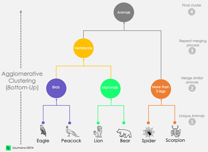
Each data point starts in its cluster.
Clusters are merged as we move up the hierarchy.
Performs well for large datasets.
Merging is based on the similarity between clusters using:
Single-linkage: Minimum distance between points in two clusters.
Complete-linkage: Maximum distance between points in two clusters.
Average linkage: Average distance between points in two clusters.
Produces a dendrogram showing the cluster hierarchy.
Steps:
Assign each point to its own cluster
Calculate the distance matrix
Merge the closest pair of clusters
Update the distance matrix
Repeat steps 3 and 4 until all points are in one cluster
Divisive Clustering (Top-Down)
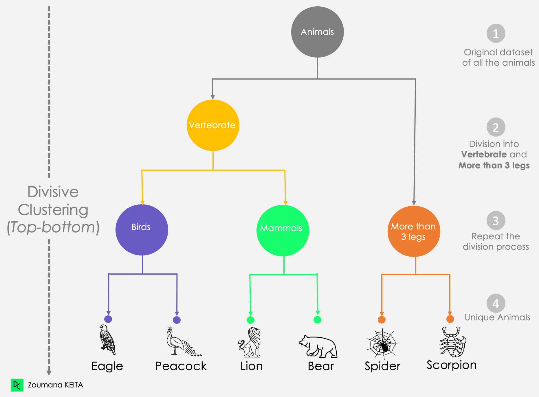
All points start in one cluster.
Splits clusters as we move down the hierarchy.
Performs poorly for large datasets due to computational complexity.
Splits are based on similarity measures like variance.
Steps:
Start with all points in one cluster
Split the cluster with the largest variance into two sub-clusters
Continue splitting clusters with the largest variance
Stop when each point is in its cluster
Partitional Algorithms
Partitional clustering algorithms partition the data into a set of disjoint clusters.
K-Means Clustering
The most popular partitional clustering algorithm.
Assumes that clusters are spherical in shape with similar spread.
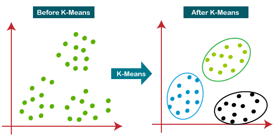
Steps:
Choose the number of clusters K
Randomly initialize K cluster centers
Assign each point to the nearest cluster centre
Recalculate the cluster centres
Repeat steps 3 and 4 until convergence.

Advantages:
Simple and easy to implement
Scales well to large datasets
Disadvantages:
Requires specifying the number of clusters K
Sensitive to initialization
Assumes spherical clusters
Expectation Maximization (EM)
Assumes that data points are generated from a mixture of underlying probability distributions (Gaussian, Poisson etc.)
Estimates model parameters using an iterative refinement technique.

Steps:
Initialize model parameters randomly
E-step: Calculate the probability that each point belongs to each cluster
M-step: Re-estimate model parameters to maximize the likelihood
Repeat the E and M steps until convergence.
Advantages:
Can estimate the number of clusters automatically.
Can handle non-spherical clusters.
Disadvantages:
Computationally expensive
Can get stuck in local optima
Clustering Large Databases
Traditional clustering algorithms do not scale well to large datasets due to their time and memory requirements. Various algorithms have been proposed to cluster large databases:
BIRCH (Balanced Iterative Reducing and Clustering using Hierarchies)
Agglomerative clustering algorithm.
Builds a CF tree (Clustering Feature tree) to cluster large amounts of numeric data.
The CF-tree summarizes subclusters using clustering features - number of points, linear sum and squared sum.
Performs clustering on a sample of the data and then assigns the remaining points.
Advantages:
Very efficient for large datasets
Can handle data streams
Disadvantage:
- Performance degrades for non-spherical clusters
Diagram and Code: Here
DBSCAN (Density-Based Spatial Clustering of Applications with Noise)
Density-based clustering algorithm.
Finds clusters based on areas of high density separated by areas of low density.
Uses two parameters - epsilon (neighbourhood radius) and minPoints (minimum number of points).
Can identify noise points and handle clusters of arbitrary shape.
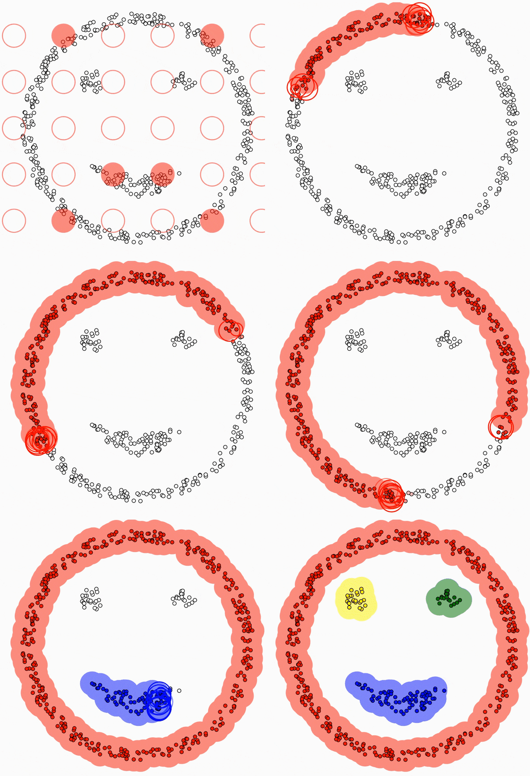
To scale to large datasets:
Use spatial indexes like R-trees to index the data
Only calculate the density for points in neighbourhoods
Advantage:
- Very efficient for clustering large spatial datasets
CURE (Clustering Using Representatives)
Agglomerative clustering algorithm.
Uses a representative set of points to summarize clusters.
The representatives are selected by shrinking each data point towards the centroid of the cluster.
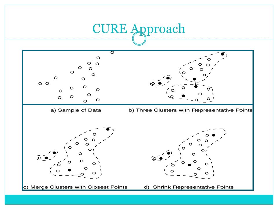
To scale to large datasets:
- Use a small representative set of points instead of all points.
Advantage:
- Can handle clusters of arbitrary shape and density.
Evaluation of Clusters
Various metrics can be used to evaluate the quality of clusters produced by clustering algorithms:
Silhouette Coefficient
Measures how closely points are grouped within a cluster compared to other clusters.
Calculates a silhouette score for each data point which ranges from -1 to 1.
A score near +1 indicates the point is well-matched to its own cluster and poorly matched to neighbouring clusters.
A score near -1 indicates the point is probably assigned to the wrong cluster.
The average of all silhouette scores is the Silhouette Coefficient for the overall clustering.
A high Silhouette Coefficient indicates a good clustering.
Davies-Bouldin Index
Measures the ratio of within-cluster distances to between-cluster distances.
Lower values of the index indicate better clustering.
Calculated as the average similarity measure between each cluster and its most similar cluster.
Smaller clusters that are well separated give a lower index.
Formula:
DB = (1/n) ∑ (i=1 to n) max (j≠i) { Ri + Rj / d(Ci , Cj) }
Where:
Ri is the within-cluster distance for cluster i
d(Ci, Cj) is the distance between clusters i and j
Association Rule Mining
Association rule mining aims to find interesting associations or correlation relationships among items in a transaction database.
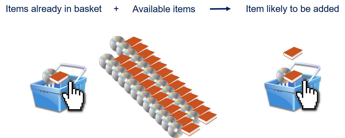
For example, in a supermarket transaction database:
80% of customers who buy milk also buy bread.
60% of customers who buy nappies also buy beer.
An association rule has two parts:
Antecedent (if)
Consequent (then)
For example:
{milk} → {bread}
{nappies} → {beer}
Two important metrics for association rules:
Support - how often the rule occurs in the dataset. Measures importance.
Confidence - how often items, in consequence, appear given items in the antecedent. Measures reliability.
For example:
Support = 20% (out of all transactions, 20% contain both milk and bread)
Confidence = 80% (out of transactions with milk, 80% also contain bread)
Popular algorithms:
Apriori - generates candidate itemsets and then scans the database to determine frequent itemsets.
FP-Growth - builds a frequent pattern tree and mines the database to find frequent itemsets.
To scale to large datasets:
Use parallel and distributed algorithms that partition the dataset across multiple machines.
Apriori and FP-Growth can both be parallelized.
Apriori Algorithm
The Apriori algorithm is a popular method for finding frequent item sets and generating association rules.
How it works
It makes multiple passes over the transaction database.
In the first pass, it counts item occurrences to find frequent 1-itemsets.
In subsequent passes, it generates candidate k-itemsets from frequent (k-1)--itemsets found in the previous pass.
It then prunes the candidates that have any subset which is not frequent.
Finally, it scans the database to determine frequent candidates among the pruned candidates.
This process repeats until no frequent k-itemsets are found.
Pseudocode
Find all frequent 1-itemsets
Join frequent k-itemsets to generate candidates for (k + 1)-itemsets
Prune (k + 1)-itemsets whose k-subsets are infrequent
Scan the database and calculate support for candidates
Return all frequent (k + 1)-itemsets
Ck: Candidate itemset of size k
Lk: frequent itemset of size k
L1 = {frequent items}; for (k = 1; Lk !=∅; k++) do begin C(k+1) = candidates generated from Lk; for each transaction t in the database do increment the count of all candidates in C(k+1) that are contained in t L(k+1) = candidates in Ck+1 with min_support end return ∪k Lk;
Pros and cons
Pros:
Simple and easy-to-understand algorithm
Guarantees to find all frequent itemsets
Cons:
Multiple passes over the dataset required
Generates a lot of candidate sets, especially for large itemsets
Performance degrades with lower minimum support
FP-Growth Algorithm
The FP-growth algorithm is an efficient method for mining frequent item sets without candidate generation.
How it works
FP-growth works by constructing a frequent pattern tree (FP-tree), which stores transaction data in a compressed form.
The root of the tree contains all frequent items. Each node represents an item and contains information about that item.
The FP-tree is constructed by first scanning the database to find frequent items. Transactions are then inserted into the tree.
Pattern growth is performed by constructing conditional FP-trees for each frequent item. These trees contain transactions that contain that item.
Frequent itemsets are generated by mining each conditional FP-tree. The itemsets found are combined with the conditional item to generate all frequent itemsets.
Pseudocode
Scan the database to find frequent items and sort them in descending order by frequency
Construct the FP-tree by inserting transactions
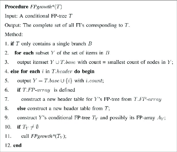
Call FP-growth on the FP-tree to generate frequent itemsets
FP-growth works as follows:
If the FP-tree contains a single path, generate itemsets from the path
Otherwise, recursively generate itemsets from conditional FP-trees
Pros and cons
Pros:
Efficient for mining frequent itemsets without candidate generation
Uses less memory than Apriori
Scales well for large datasets
Cons:
Requires sorting of items by frequency before tree construction
Performance degrades with low minimum support
Parallel and Distributed Association Rule Mining
With the advent of big data, traditional association rule mining algorithms like Apriori and FP-growth face scalability challenges. Parallel and distributed techniques are needed to mine large datasets efficiently.
MapReduce-based Apriori
MapReduce can be used to parallelize the Apriori algorithm.
In the map phase, transactions are partitioned among map tasks. Each map task finds local frequent 1-itemsets.
The reduce phase aggregates the local frequent itemsets from all maps to find global frequent 1-itemsets.
This process is repeated to find higher-order frequent itemsets.
The candidate generation and frequency counting steps of Apriori are well suited for the map and reduce functions.
Distributed FP-Growth
The FP-tree structure can be partitioned and distributed across nodes.
Each node constructs a local FP tree from its partition of the dataset.
Local frequent itemsets are found by mining each local FP-tree.
The local frequent itemsets are aggregated to find global frequent itemsets.
The conditional FP-trees can also be distributed in the same way.
This approach scales well for large datasets since the FP-tree is divided and mined in parallel.

